Auditing Racial Bias in an Employment Prediction Tool
A blog post that trains a logistic regression classifier to predict employment status and then performs an audit of the model to assess racial bias in the model. This post contains some basic exploration of the data, model training, a bias audit of the model, and a discussion of bias within the model and the ethics of employment prediction tools.
Author
Eliza Wieman
Published
April 2, 2023
Auditing Allocative Bias
In this blog post, I train a logisitc regression model to predict employment status using a variety of demographic features excluding race, and then I perform a fairness audit to assess whether the model displays racial bias. All data I use is from the American Community Survey. My blog post contains some initial basic exploration of the data, followed by model training, a fairness audit and some concluding discussion.
Choosing a Problem
For this blog post, I chose to examine racial bias in an employment status prediction model. I looked specifically at data from the state of Delaware, as this is where I am from. I trained my model on the list of features suggested in the blog post assignment, which include sex, age, level of schooling, disability status, and nativity, among other features. All features used are explained in detail in the appendix of Ding et al. After choosing my problem, I downloaded the data extracted relevant features and cleaned it up to prepare for training, and then performed a train/test split.
Now that we’ve defined a problem, let’s do some basic descriptive analysis. To do this easily, we’ll recombine our group and label data with the feature data and print them as a single dataframe.
Our dataframe has 7298 rows, corresponding to 7298 individuals. If we take the mean of the label column we see that 0.46 of the individuals in the dataset have a label of 1, meaning they are employed.
df["label"].mean()
0.45765963277610305
Next, we’ll look at the racial distribution of the dataset. We see that there are 5535 White individuals, 1168 Black/African American individuals, and 595 individuals of other self-identified racial groups. The largest racial group in the dataset by far is White individuals.
If we look at employment rate by race, we see an employment rate of 0.46 for White individuals and an employment rate of 0.44 for Black/African American individuals.
df.groupby("group")[["label"]].mean()
label
group
1
0.462511
2
0.443493
3
0.461538
5
0.300000
6
0.494382
7
1.000000
8
0.433333
9
0.358824
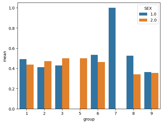
We can break this down further to look at differences in employment rate by both race and sex. We see higher employment rates for White males, compared with White females. Conversely, we see that Black females have higher employment rates than Black males. The gap between male and female employment rates is 5-6% for both racial groups.
df.groupby(["group","SEX"])[["label"]].mean()
label
group
SEX
1
1.0
0.490064
2.0
0.436890
2
1.0
0.411654
2.0
0.470126
3
1.0
0.428571
2.0
0.500000
5
1.0
0.000000
2.0
0.500000
6
1.0
0.532258
2.0
0.461538
7
1.0
1.000000
8
1.0
0.524590
2.0
0.338983
9
1.0
0.362637
2.0
0.354430
We can also visualize these trends using a barchart. From the barchart, we can see that there are not particularly large disparities in employment rate by gender for the different races, except for groups 5 and 7, which appear to only have data on females and males, respectively.
import seaborn as snsmeans = df.groupby(["group", "SEX"])["label"].mean().reset_index(name ="mean")sns.barplot(data = means, x ="group", y ="mean", hue ="SEX")
<AxesSubplot: xlabel='group', ylabel='mean'>
Choosing and Training a Model
After doing some basic exploration of the data, it is now time for us to choose and train a model. We’ll train a logistic regression model, but we’ll tune the polynomial features parameter using our training data before testing our model.
/Users/elizawieman/opt/anaconda3/envs/ml-0451/lib/python3.9/site-packages/sklearn/linear_model/_logistic.py:458: ConvergenceWarning: lbfgs failed to converge (status=1):
STOP: TOTAL NO. of ITERATIONS REACHED LIMIT.

Increase the number of iterations (max_iter) or scale the data as shown in:
    https://scikit-learn.org/stable/modules/preprocessing.html
Please also refer to the documentation for alternative solver options:
    https://scikit-learn.org/stable/modules/linear_model.html#logistic-regression
  n_iter_i = _check_optimize_result(
Polynomial degree = 2, score = 0.81
/Users/elizawieman/opt/anaconda3/envs/ml-0451/lib/python3.9/site-packages/sklearn/linear_model/_logistic.py:458: ConvergenceWarning: lbfgs failed to converge (status=1):
STOP: TOTAL NO. of ITERATIONS REACHED LIMIT.

Increase the number of iterations (max_iter) or scale the data as shown in:
    https://scikit-learn.org/stable/modules/preprocessing.html
Please also refer to the documentation for alternative solver options:
    https://scikit-learn.org/stable/modules/linear_model.html#logistic-regression
  n_iter_i = _check_optimize_result(
Polynomial degree = 3, score = 0.807
/Users/elizawieman/opt/anaconda3/envs/ml-0451/lib/python3.9/site-packages/sklearn/linear_model/_logistic.py:458: ConvergenceWarning: lbfgs failed to converge (status=1):
STOP: TOTAL NO. of ITERATIONS REACHED LIMIT.

Increase the number of iterations (max_iter) or scale the data as shown in:
    https://scikit-learn.org/stable/modules/preprocessing.html
Please also refer to the documentation for alternative solver options:
    https://scikit-learn.org/stable/modules/linear_model.html#logistic-regression
  n_iter_i = _check_optimize_result(
Polynomial degree = 4, score = 0.811
/Users/elizawieman/opt/anaconda3/envs/ml-0451/lib/python3.9/site-packages/sklearn/linear_model/_logistic.py:458: ConvergenceWarning: lbfgs failed to converge (status=1):
STOP: TOTAL NO. of ITERATIONS REACHED LIMIT.

Increase the number of iterations (max_iter) or scale the data as shown in:
    https://scikit-learn.org/stable/modules/preprocessing.html
Please also refer to the documentation for alternative solver options:
    https://scikit-learn.org/stable/modules/linear_model.html#logistic-regression
  n_iter_i = _check_optimize_result(
Polynomial degree = 5, score = 0.802
/Users/elizawieman/opt/anaconda3/envs/ml-0451/lib/python3.9/site-packages/sklearn/linear_model/_logistic.py:458: ConvergenceWarning: lbfgs failed to converge (status=1):
STOP: TOTAL NO. of ITERATIONS REACHED LIMIT.

Increase the number of iterations (max_iter) or scale the data as shown in:
    https://scikit-learn.org/stable/modules/preprocessing.html
Please also refer to the documentation for alternative solver options:
    https://scikit-learn.org/stable/modules/linear_model.html#logistic-regression
  n_iter_i = _check_optimize_result(
It seems like performance peaks around features of degree 2, so we’ll use this to train our model.
plr = poly_LR(deg =2)plr.fit(X_train, y_train)
/Users/elizawieman/opt/anaconda3/envs/ml-0451/lib/python3.9/site-packages/sklearn/linear_model/_logistic.py:458: ConvergenceWarning: lbfgs failed to converge (status=1):
STOP: TOTAL NO. of ITERATIONS REACHED LIMIT.

Increase the number of iterations (max_iter) or scale the data as shown in:
    https://scikit-learn.org/stable/modules/preprocessing.html
Please also refer to the documentation for alternative solver options:
    https://scikit-learn.org/stable/modules/linear_model.html#logistic-regression
  n_iter_i = _check_optimize_result(
In a Jupyter environment, please rerun this cell to show the HTML representation or trust the notebook. On GitHub, the HTML representation is unable to render, please try loading this page with nbviewer.org.
After fitting our model, let’s first calculate its overall accuracy on the test dataset. We get an accuracy of 0.81. This is relatively good, but I would not want to release a tool into the real-world with an accuracy this low. It could be worth exploring other models or feature combinations for training a different model in the future.
plr.score(X_test, y_test).round(4)
0.8121
Next let’s calculate positive predictive value (PPV) as well as false negative and false positive rates. To do this, we’ll extract our model’s predictions and construct a normalized confusion matrix.
We see a PPV of 0.799, meaning that approximately 80% of the individuals that our model predicted were employed are actually employed. We see relatively low FPR and FNR, with the false positive rate about 30% higher than the false negative rate. This means our model overpredicts employed status - we are more likely to predict an unemployed person is employed, rather than predicting that an employed person is unemployed.
By-Group Measures
Now let’s break things down by race, focusing specifically on the White and Black/African American groups. Looking at overall accuracy, we see that the accuracy for White indiciduals is slightly higher than Black/African American individuals, by about 3%.
df_test = pd.DataFrame(X_test, columns = features_to_use)df_test["group"] = group_testdf_test["label"] = y_testblack_ix = df_test["group"] ==2white_ix = df_test["group"] ==1correct_pred = y_pred == df_test["label"]# accuracy on Black defendantsaccuracy_black = correct_pred[black_ix].mean()# accuracy on white defendantsaccuracy_white = correct_pred[white_ix].mean()print("White accuracy: ", accuracy_white)print("Black accuracy: ", accuracy_black)
White accuracy:  0.817117776152158
Black accuracy:  0.7911392405063291
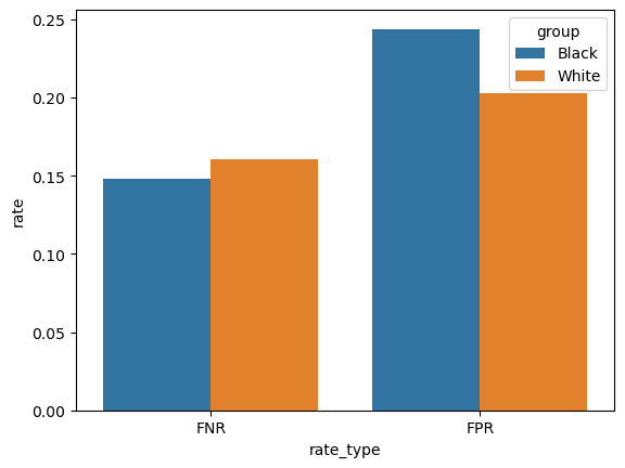
Next we’ll break down PPV, FPR and FNR by group. We see that false positive rates are higher than false negative rates across both groups, but the gap between FPR and FNR is much larger for Black individuals (10% versus 4%).
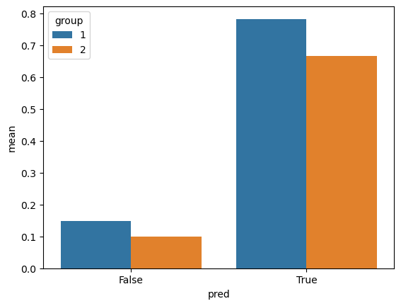
Now we’ll examine some specific bias measures. First let’s check if our model is well calibrated. To do this, we’ll check if the fraction predicted employed people who are actually employed is the same across groups. Of those predicted employed, slightly more White than black individuals were actually employed, but the rates are relatively consistent across groups.
df_test["pred"] = y_preddf_test = df_test[white_ix|black_ix]means = df_test.groupby(["group", "pred"])["label"].mean().reset_index(name ="mean")p = sns.barplot(data = means, x ="pred", y ="mean", hue ="group")
Error Rate Balance
To determine error rate balance, we’ll check if FPR and FNR are consistent across both groups. We already calculated false positive and false negative rates by group above, and we can see that they differ slightly, but not substantially. We can plot these trends also to visualize them better. False negative rates are pretty consistent across the two groups, but the false positive rate for Black/African-American individuals is higher than for White individuals.
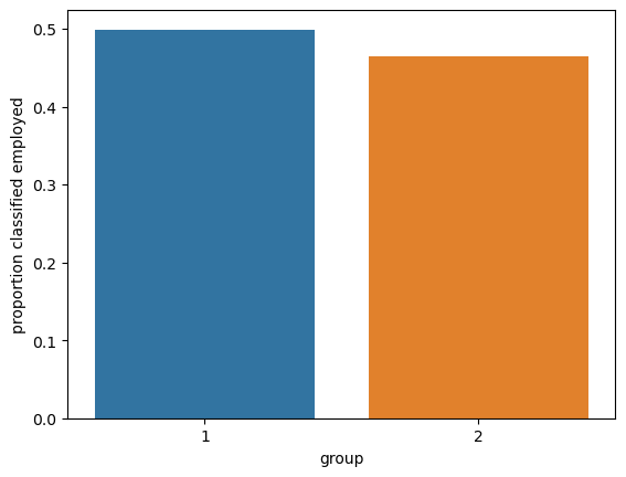
To calculate statistical parity, we check if the proportion of individuals classified as employed is the same across groups. While the rates differ slightly, they are close enough that we can probably say statistical parity is satisfied.
means = df_test.groupby("group")["pred"].mean().reset_index(name ="proportion classified employed")print(means)p = sns.barplot(data = means, x ="group", y ="proportion classified employed")
   group  proportion classified employed
0      1                        0.498903
1      2                        0.465190
Discussion
An employment prediction tool such as the model trained here could be useful for a variety of companies. For example, companies trying to recruit employees could use an employment prediction tool to find unemployed people to target for recruiting. Employment is also often used as a proxy for wealth/financial stability, so people trying to assess someone’s financial stability, such as a bank considering someone for a loan or a landlord considering someone for a lease might use an employment prediction tool when evaluating them. This could negatively impact people who were predicted as unemployed, particularly if they actually were employed, preventing them from needed opportunities for financial growth. Based on my bias audit, White individuals are more often predicted as employed than Black individuals. However, White individuals are less likely to be falsely predicted as employed than Black people are, while White people are slightly more likely to be falsely predicted as unemployed than Black people are. Thus, if my model was used as an employment prediction tool by banks, landlords, etc., it would probably approve slightly more White people for loans and leases than Black people. This could reinforce existing societal biases within the US which give White people more access to capital and opportunities for financial growth. On the other hand, the higher FPR for Black individuals could allow unemployed Black people to still have access to new sources of capital, housing, etc. If used as a recruiting tool, the higher FPR for Black individuals would intorduce additional hurdles for raising the employment rate among Black people because recruitment efforts would be more likely to be targeted towards White people.
Based on my audit, I do not think that my model shows significant problematic bias. The model is relatively well-calibrated for race and it satisfies statistical parity. The one area where the model appears to be a bit biased is in error rate balance, specifically with regard to false positive rates. It is surprising to me that the FPR is higher for Black people than White people, as it is contrary to existing societal biases. While more balanced false positive rates would be preferred, a difference in 4% does not seem too problematic. Additionally, I think that it is better for this model to have inflated false positive rates, rather than false negative rates, as false positive rates would give people more opportunities to accrue capital, rather than less. Despite the model not showing much racial bias, I still do not think that employment prediction tools should be used. If a person is not required to divulge their employment status for a certain application process, then I do not think that their assumed employment status should be allowed to be considered. While employment prediction tools could be helpful for recruiting purposes, I think they are likely to do more harm than good in gatekeeping people from access to housing, money, and other living needs. I do not see enough positive uses for these tools that outweigh the potential negative impacts, so I think that their use should be banned.